The economics of route density

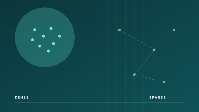
If you want to understand why one last-mile operation makes money and another does not, start with a single number: stops per kilometre driven. Almost everything else — fuel, driver hours, vehicle count, even first-attempt success — flows from how tightly your deliveries cluster in space and time. We call it route density, and it is the most important metric most operators never put on a dashboard.

Why density dominates the cost model

Break a delivery route into its two parts. There is driving — the time and distance between stops — and there is servicing — parking, walking to the door, the handover, getting a signature, walking back. On a sparse rural route, driving dominates: a courier might spend most of the day behind the wheel to make forty drops. On a dense urban route, servicing dominates: the van barely moves, but the courier makes a hundred and twenty drops because the next door is thirty metres away.

The cost per parcel is roughly the cost of the route divided by the stops on it. A route costs about the same to run whether it holds sixty stops or ninety — the driver is paid for the shift either way, the van is leased by the month either way. So when you add stops to an existing route without extending it much, the cost of each parcel falls. That is the whole game. Density is not a nice-to-have; it is the denominator.

Here is the part that surprises people. The relationship is not linear. Going from 40 to 50 stops on a route is a meaningful saving. Going from 90 to 100 is enormous, because you are spreading a nearly fixed cost across more and more parcels while the marginal driving distance between adjacent stops keeps shrinking. Density has increasing returns, right up until the point the driver runs out of hours in the shift.

The measurement mistake

Most operators, if they track density at all, track it as an average across the whole operation: total stops divided by total kilometres, one number for the week. That number is nearly useless, because it blends your excellent dense routes with your terrible sparse ones and hides both.

Density is a property of an individual route on an individual day, and it is shaped by decisions you make before the van leaves: how you carve the territory into rounds, which orders you accept for which day, whether you let customers pick any two-hour slot or nudge them toward the ones that fit an existing route. Average density tells you nothing about those decisions. Per-route density, plotted as a distribution, tells you everything — it shows you the long tail of sparse routes that are quietly eating your margin.

The question is never "what is our density?" It is "which routes are below the line, and why did we build them that way?"

What actually moves density

Once you measure it per route, the levers become obvious. In our experience four of them do most of the work.

Territory design. Fixed delivery zones drawn on a map years ago almost never match today's order pattern. E-commerce demand shifts neighbourhood by neighbourhood as new residential blocks fill up. Redrawing zones against recent demand — or letting the planner draw them fresh each day — is often the single biggest one-time gain, worth ten to fifteen percent on its own.

Time-window discipline. Every promised delivery window is a constraint that fragments a route. A customer who insists on 09:00–11:00 in a neighbourhood you otherwise serve in the afternoon forces either a detour or a whole extra pass. You do not have to abolish windows — you have to price them, and steer demand toward the windows that fit routes you are already running. A grocery checkout that gently highlights the "green" slot is doing density engineering, whether the retailer calls it that or not.

Order acceptance and cut-offs. Which orders you commit to which day is a density decision made a day early. Pulling a cut-off forward by two hours can let the planner see the whole picture before it commits, instead of stapling late orders onto routes that are already fixed.

Channel mix. A parcel diverted to a locker is not a stop on a doorstep route at all — it is one stop at a cabinet that clears twenty parcels at once. Every locker-eligible parcel you move off the van raises the effective density of what remains. This is why locker strategy and route density are the same conversation.

The rural exception

None of this repeals geography. Some routes will always be sparse, because the customers are genuinely far apart. In the Baltics this is a real and permanent feature: a route around Kaunas behaves nothing like a route through the villages east of Utena. The mistake is not having sparse routes; it is planning them with the same assumptions as dense ones, and pricing them as if they cost the same. For genuinely sparse territory, the right answers are different — less frequent service, locker consolidation points, or a delivery-day model rather than a next-day promise.

Start with the distribution

If you take one thing from this: stop looking at your average. Pull last month's routes, compute stops per kilometre for each one, and plot them. The shape of that distribution — how long the sparse tail is, how much volume sits in it — is the clearest picture of your last-mile economics you will ever get, and it usually points straight at the fix. It is the first thing our planner shows a new customer, and it is almost always the moment the conversation gets serious.